Support Vector Machines (SVM)

This blog post is part of a series, where I talk about concepts and algorithms in Machine Learning. In this part I want to talk about another popular algorithm, which is widely used for solving classification and regression problems. I am of course talking about Support Vector Machines (SVM).

What does Support Vector Machines do?

Support Vector Machines are supervised learning models for classification and regression problems. They can solve linear and non-linear problems and work well for many practical problems. The idea of Support Vector Machines is simple: The algorithm creates a line which separates the classes in case e.g. in a classification problem. The goal of the line is to maximizing the margin between the points on either side of the so called decision line. The benefit of this process is, that after the separation, the model can easily guess the target classes (labels) for new cases.

Maybe you say now, that this probably only works for a low dimensional problem, e.g a data set with only 2 features, but that is wrong! Support Vector Machines are actually very effective in higher dimensional spaces. It is even very effective on data sets where number of dimensions is greater than the number of samples. This is mainly because of the kernel trick, which we talk about it later. Further advantages of Support Vector Machines are the memory efficiency, speed and general accuracy in comparison to other classification methods like k-nearest neighbor or deep neural networks. Of course they are not every time better than e.g. deep neural networks, but sometimes they still outperform deep neural networks.

Difference between Linear and Non-Linear Data

To clear everything up, I explain quickly what it is all about the linear and non-linear data thing. We talk about linear data, when we can classify the data with a linear classifier. The linear classifier makes his classification decision based on a linear combination of characteristics. The characteristics are also known as features in machine learning. The following picture will make things more clear.

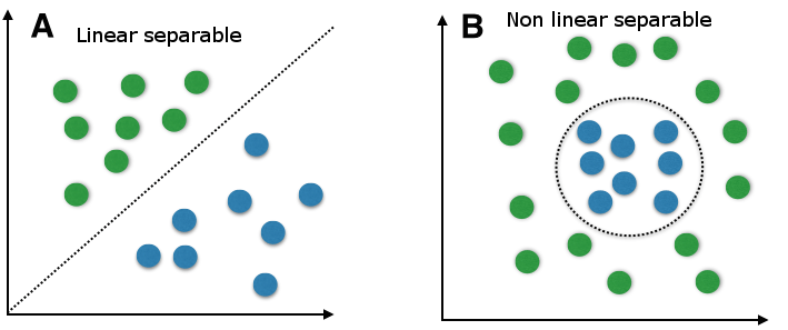
In figure A we can separate the target labels linear with a line (like Support Vector Machines do classification with a decision line). A linear classifier can do this with a linear combination of characteristics. We could use e.g. Support Vector Machines do build a model, but we could also use many other linear classification methods like quadratic classification.

In figure B we can not separate the target labels linear. The data is more complex divided. Therefore we can not just use a linear classification method. Fortunately Support Vector Machines can do both, linear and non-linear classification. Lets first take an easier linear example to get an introduction about Support Vector Machines. Later we will look at non-linear classification with Support Vector Machines and we will see how it works with the kernel trick.

Linear Example

To create an linear example and train a model with the Support Vector Machines algorithm I will use the C-Support Vector Classification algorithm from the sklearn library in Python. First we will just implement the clean C-Support Vector Classification algorithm (SVC) on the iris data set.

# iris_svc.py
# iris dataset
# 150 total entries
# features are: sepal length in cm, sepal width in cm, petal length in cm, petal width in cm\n 
# labels names: setosa, versicolor, virginica
#
# used algorithm: SVC (C-Support Vector Classifiction) 
#
# accuracy ~100%
#
from time import time
import numpy as np
from sklearn.datasets import load_iris
from sklearn import svm
from sklearn.metrics import accuracy_score
def main():
	data_set = load_iris()
	features, labels = split_features_labels(data_set)
	train_features, train_labels, test_features, test_labels = split_train_test(features, labels, 0.18)
	print(len(train_features), " ", len(test_features))
	clf = svm.SVC()
	print("Start training...")
	tStart = time()
	clf.fit(train_features, train_labels)
	print("Training time: ", round(time()-tStart, 3), "s")
	print("Accuracy: ", accuracy_score(clf.predict(test_features), test_labels))


def split_train_test(features, labels, test_size):
	total_test_size = int(len(features) * test_size)
	np.random.seed(2)
	indices = np.random.permutation(len(features))
	train_features = features[indices[:-total_test_size]]
	train_labels = labels[indices[:-total_test_size]]
	test_features  = features[indices[-total_test_size:]]
	test_labels  = labels[indices[-total_test_size:]]
	return train_features, train_labels, test_features, test_labels
def split_features_labels(data_set):
	features = data_set.data
	labels = data_set.target
	return features, labels
if __name__ == "__main__":
	main()

Output:

123 27
Start training…
Training time: 0.002 s
Accuracy: 1.0

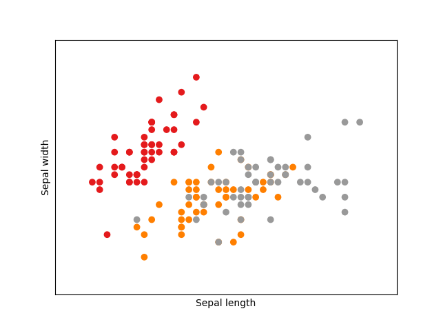
Okay, this seems to work pretty well, but how does a decision line of a Support Vector Machine looks like? First lets plot the iris data set to see how the data set looks like. To make things easier, lets just concentrate on the first two features: sepal length and sepal width.

With the Support Vector Machine algorithm we could probably separate now the red group from the other two groups (orange and grey).

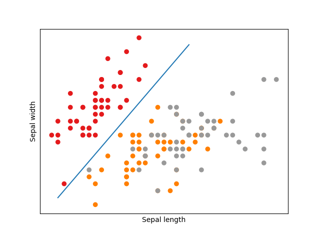
So this would probably look like this. But we still have the problem, that the orange and grey group are difficult to separate. We could guess, that a higher sepal width and a higher sepal length is a sign, that the entry is from the grey group, but fortunately we do not have to assume such things, because we have a third feature and a fourth features, petal length and petal width, so that we can group them with decision lines in higher dimensions. The example above should show the general principle of Support Vector Machines. Here we do not have a binary classification problem (2 labels), but we can easily separate the red group from the grey and orange group by a decision line by using only two features out of four features.

How does this work?

For humans this seems pretty intuitive. We just drawing a line to separate the different labeled classes from each other. But how does Support Vector Machines solve this problem? The SVM want to find are so called maximum-margin hyperplane.

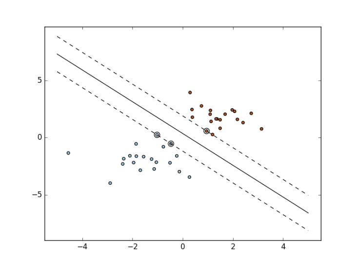
The hyperplane is the line with the biggest margin to both groups. We have called the line above decision line, but the mathematical correct term is hyperplane, because in dimensions higher than two, it will be not a line anymore. We will give the Support Vector Machine algorithm a bunch of labeled vectors as a training set. All vectors are p dimensional, p is the number of features we have in our training set. To find the maximum margin hyperplane, we have to maximize the margin to every nearest point of each target group. In a binary classification, we can declare the labels of the two target groups as -1 and 1. The hyperplane as a set of points can be described as

where x is the normal vector to the hyperplane and b is a bias. A normal vector simply is an orthogonal standing vector to a line or plane. If you are familiar with linear algebra, this may look familiar to you. It is like the Hesse normal form, except that w does not have to be a unit vector. The parameter determines the offset of the hyperplane from the origin along the normal vector . With the use of the hyperplane (decision line) the model can now classify new entries.

There are actually different sub classifier, who behave different. The Soft Margin Classifier allows some noise in the training data, but on the other side the Hard Margin Classifier does not allow noise in the training data.

Using the Support Vector Machines for non-linear data with the kernel trick

Until know we have talked about linear examples and how Support Vector Machines work and how you can implement them with sklearn in Python. I already talked a little bit about non-linear data. When there is a non-linear data set Support Vector Machines can not simply draw a linear hyperplane. Therefore Support Vector Machines use the kernel trick. When you have non-linear data, the kernel method helps you to find pattern and relations to reach a high accuracy in your final machine learning model.

How does the Kernel method works?

The kernel method are contains are so called kernel function. These function map the non-linear separable input space into a higher dimensional linear separable feature space. And in this new higher dimensional linear separable feature space Support Vector Machines can work as normal. The kernel method then maps the solutions back, so that in the non-linear separable input space you then have a non-linear solution.

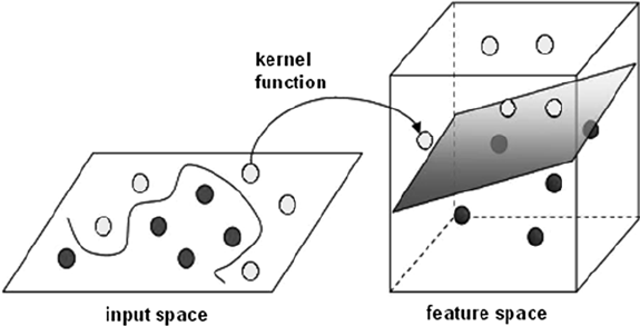
In the example above we have a two dimensional feature space, which is non-linear. With the kernel function we can map the input space into a three dimensional feature space. In this feature space we then can separate the training set linear. When we map the solution back to the input space we get a non-linear solution.

Implementation

In sklearn you can use different kernels to train your model. You can check out here how you implement a non-linear Support Vector Machine classifier in Python. There is no big difference to the linear example above, you just have to figure out what parameters you want to choose to get an high accuracy for your machine learning model.

Resume

Support Vector Machines calculate a hyperplane to build a classification model. The hyperplane divides the target labels with a maximized margin. With the use of the kernel trick you also can classify non-linear data.