TIL: Minimizing cost functions with gradient descent

Today I learned about gradient descent and how you can minimize cost function for liner regression problems with gradient descent.

In yesterdays TIL I wrote about linear regression and cost functions (also known as MSE) for measuring the accuracy of a hypothesis in linear regression problems.

So what is a gradient descent? With gradient descent you can minimize a cost function by finding the local minimum. Essentially gradient descent figures out which s we have to choose for optimizing our hypothesis. The gradient descent algorithms is as following:

repeat until convergence:

J = 0,1 representing the feature index numbers. For each iteration every should update simultaneously.

represents the learning rate. If the learning rate is to large, gradient descent can overshoot the minimum and might not able to find it. If the learning rate is to small, gradient descent can be slow.

is our derivative.

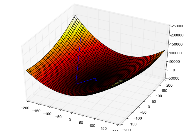
The following figure shows an example of gradient descent. The x and z axis are s and the y axis is the value of our cost function J of our hypothesis h. With each iteration our hypothesis changes and we approximate at the local minimum.

Written on May 1st , 2018 by Lasse Schultebraucks